Flexible Indexes: Exciting new ways to slice and dice your data!
Monday, August 11th, 2025 (23 days ago)
TL;DR: over the last few years Xarray has been through a gradual although major refactoring of its internals that makes coordinate-based data selection and alignment customizable. Xarray>=2025.6 now enables more efficient handling of both traditional and more exotic data structures. In this post we highlight a few examples that take advantage of this new superpower! See the Gallery of Custom Index Examples for more!
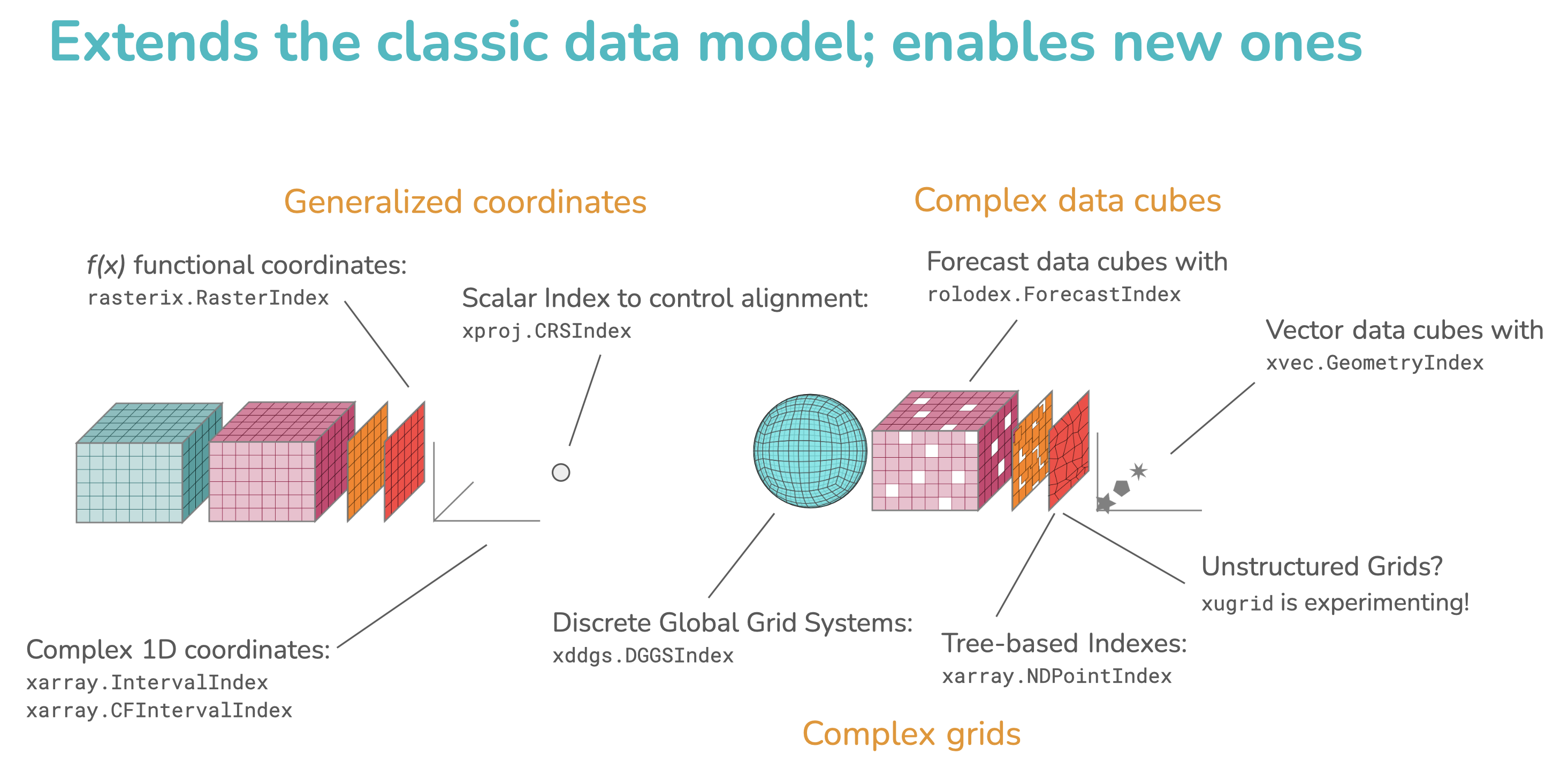
Summary schematic from our 2025 SciPy Presentation highlighting new custom Indexes and usecases. Link to full slide deck
Indexing basics#
First thing's first, what is an Index and why is it helpful?
In brief, an index makes data retrieval and alignment more efficient. Xarray Indexes connect coordinate labels to associated data location (array indices) and encode important contextual information about the coordinate space.
Examples of indexes are all around you and are a fundamental way to organize and simplify access to information.
In the United States, if you want a book about Natural Sciences, you can go to your local library branch and head straight to section 500. Or if you're in the mood for a classic novel go to section 800. Connecting thematic labels with numbers ({'Natural Sciences': 500, 'Literature': 800}) is a classic indexing system that's been around for hundreds of years (Dewey Decimal System, 1876).
The need for an index becomes critical as the size of data grows - just imagine the time it would take to find a specific novel amongst a million uncategorized books!
The same efficiencies arise in computing. Consider a simple 1D dataset consisting of measurements M=[10.0,20.0,30.0,40.0,50.0,60.0] at six coordinate positions X=[1, 2, 4, 8, 16, 32]. What was our measurement at X=8?
To answer this in code, we could either do a brute-force linear search (or binary search if sorted) through the coordinates array, or we could build a more efficient data structure designed for fast searches --- an Index. A common convenient index is a key:value mapping or "hash table" between the coordinate values and their integer positions i=[0,1,2,3,4,5]. Finally, we are able to identify the index for our coordinate of interest (X[3]=8) and use it to lookup our measurement value M[3]=40.0.
💡 Note: Index structures present a trade-off: they are a little slow to construct but much faster at lookups than brute-force searches.
pandas.Index#
Xarray's label-based selection allows a more expressive and simple syntax in which you don't have to think about the index (da.sel(x=8)). Up until now, Xarray has relied exclusively on pandas.Index, which is still used by default:
1x = np.array([1, 2, 4, 8, 16, 32]) 2y = np.array([10, 20, 30, 40, 50, 60]) 3da = xr.DataArray(y, coords={'x': x}) 4da 5
1da.sel(x=8) 2# 40 3
Alternatives to pandas.Index#
There are many different indexing schemes and ways to generate an index. A basic approach is to run a loop over all coordinate values to create an index:coordinate mapping, optionally identifying duplicates and sorting along the way. But, you might recognize that our example coordinates above can in fact be represented by a function X(i)=2**i where i is the integer position! Given that function we can quickly get measurement values at any coordinate: Y(X=8) = Y[log2(8)] = Y[3]=40. Xarray now has a CoordinateTransformIndex to handle this type of on-demand calculation of coordinates!
xarray RangeIndex#
A simple special case of CoordinateTransformIndex is a RangeIndex where coordinates can be defined by a start, stop, and uniform step size. pandas.RangeIndex only supports integers, whereas Xarray handles floating-point values. Coordinate look-up is performed on-the-fly rather than loading all values into memory up-front when creating a Dataset, which is critical for the example below that has a coordinate array of 7 terabytes!
1from xarray.indexes import RangeIndex 2 3index = RangeIndex.arange(0.0, 1000.0, 1e-9, dim='x') # 7TB coordinate array! 4ds = xr.Dataset(coords=xr.Coordinates.from_xindex(index)) 5ds 6
Selection with slices preserves the RangeIndex and does not require loading all the coordinates into memory.
sliced = ds.isel(x=slice(1_000, 50_000, 100)) sliced.x
Third-party custom Indexes#
In addition to a few new built-in indexes, xarray.Index provides an API that allows dealing with coordinate data and metadata in a highly customizable way for the most common Xarray operations such as sel, align, concat, stack. This is a powerful extension mechanism that is very important for supporting a multitude of domain-specific data structures.
rasterix RasterIndex#
Earlier we mentioned that coordinates often have a functional representation.
For 2D raster images, this function often takes the form of an Affine Transform.
The rasterix library extends Xarray with a RasterIndex which computes coordinates for geospatial images such as GeoTiffs via Affine Transform.
Below is a simple example of slicing a large mosaic of GeoTiffs without ever loading the coordinates into memory:
1# 811816322401 values! 2import rasterix 3 4#26475 GeoTiffs represented by a GDAL VRT 5da = ( 6 xr.open_dataarray( 7 "https://opentopography.s3.sdsc.edu/raster/COP30/COP30_hh.vrt", 8 engine="rasterio", 9 parse_coordinates=False, 10 ) 11 .squeeze() 12 .pipe(rasterix.assign_index) 13) 14da 15
After the slicing operation, a new Affine is defined. For example, notice how the origin changes below from (-180.0, 84.0) -> (-122.4, -47.1), while the spacing is unchanged (0.000277).
1print('Original geotransform:\n', da.xindexes['x'].transform()) 2da_sliced = da.sel(x=slice(-122.4, -120.0), y=slice(-47.1,-49.0)) 3print('Sliced geotransform:\n', da_sliced.xindexes['x'].transform()) 4
1# Original geotransform: 2Affine(0.0002777777777777778, 0.0, -180.0001389, 3 0.0, -0.0002777777777777778, 84.0001389) 4 5# Sliced geotransform: 6Affine(0.0002777777777777778, 0.0, -122.40013889999999, 7 0.0, -0.0002777777777777778, -47.09986109999999) 8
XProj CRSIndex#
"real-world datasets are usually more than just raw numbers; they have labels which encode information about how the array values map to locations in space, time, etc." -- Xarray Documentation
We often think about metadata providing context for measurement values but metadata is also critical for coordinates! In particular, to align two different datasets we must ask if the coordinates are in the same coordinate system. In other words, do they share the same origin and scale?
There are currently over 7000 commonly used Coordinate Reference Systems (CRS) for geospatial data in the authoritative EPSG database!
And of course an infinite number of custom-defined CRSs.
xproj.CRSIndex gives Xarray objects an automatic awareness of the coordinate reference system so that operations like xr.align() raises an informative error when there is a CRS mismatch:
1from xproj import CRSIndex 2lons1 = np.arange(-125, -120, 1) 3lons2 = np.arange(-122, -118, 1) 4ds1 = xr.Dataset(coords={'longitude': lons1}).proj.assign_crs(crs=4267) 5ds2 = xr.Dataset(coords={'longitude': lons2}).proj.assign_crs(crs=4326) 6ds1 + ds2 7
1MergeError: conflicting values/indexes on objects to be combined for coordinate 'crs' 2
XVec GeometryIndex#
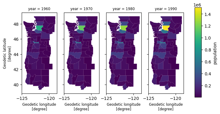
A "vector data cube" is an n-D array that has at least one dimension indexed by an array of vector geometries.
With the xvec.GeometryIndex, Xarray objects gain functionality equivalent to geopandas' GeoDataFrames!
For example, large vector cubes can take advantage of an R-tree spatial index for efficiently selecting vector geometries within a given bounding box.
Below is a short code snippet which automatically uses R-tree selection behind the scenes:
1import xvec 2import geopandas as gpd 3from geodatasets import get_path 4 5# Dataset that contains demographic data indexed by U.S. counties 6counties = gpd.read_file(get_path("geoda.natregimes")) 7 8cube = xr.Dataset( 9 data_vars=dict( 10 population=(["county", "year"], counties[["PO60", "PO70", "PO80", "PO90"]]), 11 unemployment=(["county", "year"], counties[["UE60", "UE70", "UE80", "UE90"]]), 12 ), 13 coords=dict(county=counties.geometry, year=[1960, 1970, 1980, 1990]), 14).xvec.set_geom_indexes("county", crs=counties.crs) 15cube 16
1# Efficient selection using shapely.STRtree 2from shapely.geometry import box 3 4subset = cube.xvec.query( 5 "county", 6 box(-125.4, 40, -120.0, 50), 7 predicate="intersects", 8) 9 10subset['population'].xvec.plot(col='year'); 11
Even more examples!#
Be sure to check out the Gallery of Custom Index Examples for more detailed examples of all the indexes mentioned in this post and more!
What's next?#
While we're extremely excited about what can already be accomplished with the new indexing capabilities, there are plenty of exciting ideas for future work.
Have an idea for your own custom index? Check out this section of the Xarray documentation.
Acknowledgments#
This work would not have been possible without technical input from the Xarray core team and community! Several developers received essential funding from a CZI Essential Open Source Software for Science (EOSS) grant as well as NASA's Open Source Tools, Frameworks, and Libraries (OSTFL) grant 80NSSC22K0345.